 img-buffer-etfs1-4
The upside cap in all Buffer ETF offerings, regardless of the level of downside protection, is mostly influenced by two factors: interest rates and volatility. Obviously, an investor considering an allocation in a Buffer ETF wants the highest upside cap possible during the outcome period. A high upside cap allows an investor to participate in gains to the fullest extent possible. However, there are times when upside caps can be relatively low and other times when they are well above the historical average annual return of the stock market (10%). Let’s look at how interest rates and volatility influence the upside caps of Buffer ETFs.
Interest Rates
An increase in interest rates will drive up call premiums and cause put premiums to decrease. Call options are positively influenced by an increase in interest rates and puts are negatively influenced.
To understand why, you need to think about the effect of interest rates when comparing an option position to simply owning a stock or stock index. Since it is much cheaper to buy a call option than 100 shares of a stock, a call buyer is willing to pay more for an option when interest rates are relatively high. The reason is the investor can invest the difference in the capital required between the two positions.
Let’s look at some comparative examples that make it easier to understand why interest rates positively influence call options and negatively impact put options.
Source: Shobhit Seth, Investopedia
Rising interest rates positively impact call options
Purchasing 100 shares of a stock trading at $100 will require $10,000, which, assuming a trader borrows money for trading, will lead to interest payments on the borrowed capital. Purchasing the call option at $12 in a lot of 100 contracts will cost only $1,200, yet the profit potential will remain the same as that of the long stock position.
Effectively, the differential of $8,800 will result in savings of outgoing interest payments on this loaned amount. In addition, the saved capital of $8,800 can be kept in an interest-bearing account and will result in interest income. A 5% risk-free interest rate will generate $440 in one year.
Therefore, an increase in interest rates will lead to saving in outgoing interest on the loaned amount and an increase in the amount of interest income on the savings account. Both will be positive for call option pricing. Effectively, a call option’s price increases to reflect this benefit from increased interest rates.
Rising interest rates negatively impact put options
Theoretically, shorting a stock with the objective of benefitting from a price decline, will bring in cash to the short seller. Buying a put has a similar benefit from price declines, but comes at a cost as the put option premium must be paid. This case has two different scenarios: cash received by shorting a stock can earn interest for the trader, while cash spent in buying puts is interest payable (assuming the trader is borrowing money to buy puts).
With an increase in interest rates, shorting stock becomes more profitable than buying puts, as the former generates income and the latter does the opposite. Thus, put option prices are impacted negatively by rising interest rates.
Volatility
When markets are volatile, it simply means returns are going to be volatile too, in either direction, up or down. It also means the level of uncertainty is high and this positively impacts the value of both call and put options. Call and put options actually gain in value when volatility increases. Only market volatility impacts call and put options in the same direction.
When markets are in a downtrend, volatility generally increases. Conversely, market uptrends usually cause volatility to fall. Higher volatility indicates that greater option price movement is expected in the future.
Higher volatility means greater upside risk, but higher downside risk too. This rule applies to both call and put options. This is why higher volatility makes both call and put options more valuable.
As volatility increases, the prices of all options – both calls and puts and at all strike prices – tend to rise. The greater volatility increases the chances of all options finishing in-the-money, therefore making all options more valuable.
Option pricing is a complex process. Multiple factors impact option valuations, which can lead to very high variations in option prices over the short term. Call and put option premiums are impacted inversely as interest rates change. However, volatility will positively impact both call and put prices.
15% Buffer ETF Cap Levels (2018-2023)
The graph shows the brief history of the upside caps of a 15% Buffer ETF relative to one-year U.S. Treasury yields. Less than two years after Innovator’s launch of Buffer ETFs in 2018, Treasury yields plummeted, putting downward pressure on cap levels. As rates moved higher in 2022, the caps also moved higher. The increased volatility of the 2022 bear market also contributed to the rise in upside cap levels. The 15% Buffer ETF cap level peaked at 20.70% on the reset day (September 30, 2022) for POCT (Innovator U.S. Equity Power Buffer ETF – October). Since then, cap levels have generally come down as market volatility decreased and interest rates stabilized.
15% Buffer ETF: Historical Caps vs. One-Year U.S. Treasury Yields
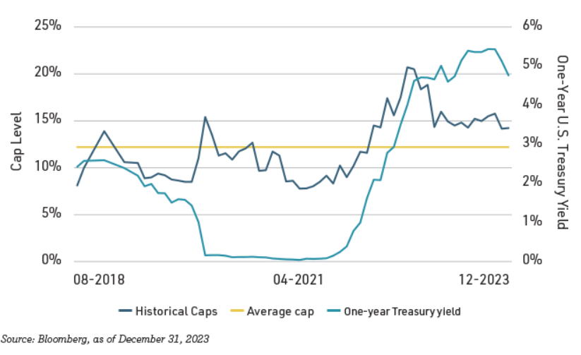
The relatively high upside caps available during both 2022 and 2023 provided an attractive risk vs. reward opportunity for investors looking for a defined level of downside protection, but also with compelling upside profit potential.
If you’re comparing Buffer ETFs that provide different levels of downside protection, it’s important to consider if the upside caps are high enough to forgo the extra protection. For example, you should compare the cap levels of a 10% Buffer series to a 15% Buffer series, with the same reset date, before purchasing either one. Do you want 5% less downside protection, and is the upside cap high enough to warrant less protection?
Let’s compare the cap levels for Buffer ETFs that provide minimal, moderate and deep protection.
How much higher is the upside cap typically for a 10% Buffer ETF vs. a 15% Buffer ETF?
FT Vest January 2024 Buffer ETFs provide a good reference for comparison:
FJAN (10% buffer) = 14.85% upside cap (net)
GJAN (15% buffer) = 12.11% upside cap (net)
If you opt for the 10% buffer, your potential upside participation is approximately 23% higher than the Buffer ETF that provides 15% downside protection. The less protection you purchase, the higher the upside cap. If the reference asset performs well during the outcome period, you would obviously participate more fully in the upside by owning FJAN, rather than GJAN. But, with FJAN you’re only protected on the first 10% loss (before fees) during the outcome period.
How do the upside caps on Deep Buffer ETFs compare to Buffer ETFs offering less protection?
The Buffer ETFs offered by FT Vest in January 2024 provide a helpful comparison:
FJAN (10% buffer) = 14.85% upside cap (net)
GJAN (15% buffer) = 12.11% upside cap (net)
DJAN (25% buffer) (-5% to -30%) = 13.09% upside cap (net)
You can see the upside caps on the Buffer series that offer 15% and 25% protection are very similar. How does the Deep Buffer ETF offer a slightly higher upside cap while protecting against nearly 2x the loss? Buffer ETF issuers obtain a competitive upside cap with a Deep or Ultra Buffer ETF by giving up protection on the first 5% loss.
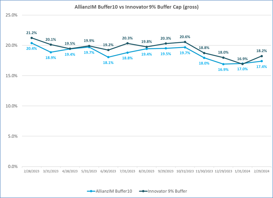
9% vs. 10% Downside Protection
Perhaps a more difficult decision is when you are considering Buffer ETFs that offer very similar levels of downside protection with only slightly different upside caps.
The graph shows a comparison of the cap levels of Innovator’s 9% Buffer series vs. Allianz’s 10% Buffer series over the past 12 months (2/28/2023 – 2/29/2024). The 9% Buffer series has provided a higher cap of approximately 0.70%, on average, with 1% less downside protection.
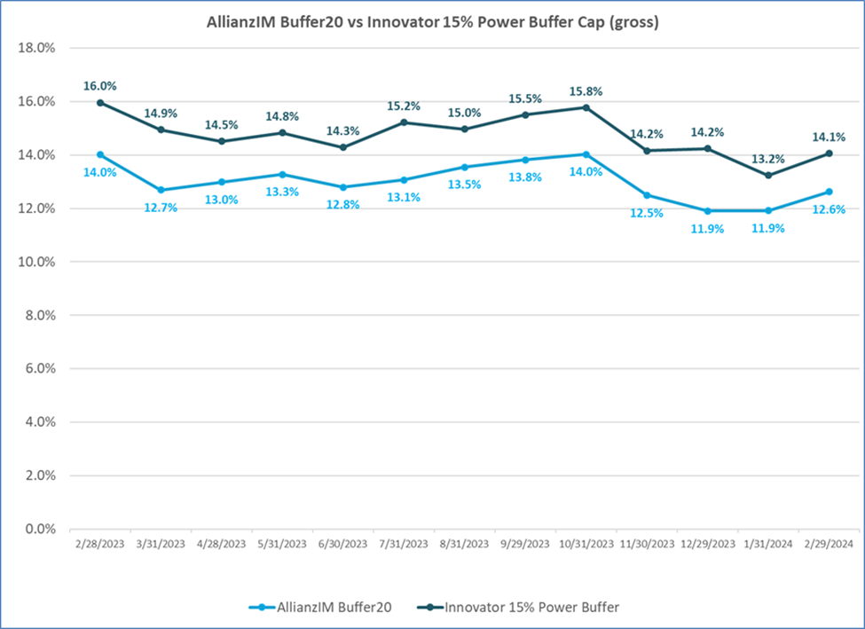
15% vs. 20% Downside Protection
There is a fairly significant difference in the cap levels and downside protection for Innovator’s U.S. Equity Power Buffer ETFs with 15% downside protection vs. Allianz’s 20 Buffer ETFs with 20% downside protection. As you can see in the graph, the cap difference has been 1.7%, on average, over the past 12 months (2/18/2023 – 2/29/2024). The 15% Power Buffer ETFs have provided a higher average cap of 1.7%, but with 5% less protection. Put differently, an investor has received more than twice as much extra protection (5% more), on average, with the Allianz 20 series, for the potential amount of upside forfeited (1.7% less).
Over the past 12 months the extra 5% protection provided by Allianz’s 20 series was obviously not needed since we’ve been in a strong market. In a bull market, investors will no doubt prefer to own a Buffer ETF that provides 15% downside protection vs. 20% protection, given the average cap has been 1.7% higher. However, whenever the next bear market hits, the extra 5% downside protection provided by Allianz’s 20 series should be comforting.
Before making a Buffer ETF purchase, it’s advisable to compare the upside cap levels to the various levels of downside protection you are considering. The cap levels can vary significantly for Buffer ETFs offering different levels of protection. While a higher cap can be enticing, it’s wise to first consider your risk profile and focus on how much downside protection you need to invest comfortably. Don’t let greed influence you to choose less protection for a higher upside cap. Your chosen level of downside protection should fit your risk profile.
Allianz has recently launched Buffer ETFs that track the SPDR S&P 500 ETF Trust (SPY), and reset every six months with a 10% buffer. Most Buffer ETFs have a 12-month outcome period, so let’s look at some potential advantages and disadvantages of a 6-month vs. a 12-month reset.
Potential advantages of a 6-month vs. 12-month outcome period:
1. There are more frequent resets with a 6-month outcome period. The buffer level is reset twice per 12-month period, which provides a fresh buffer sooner and a new upside cap too.
2. The shorter outcome period can be helpful for active investors that seek positioning over shorter time periods.
3. A Buffer ETF with a 6-month reset will typically track the reference asset more closely than the 12-month version with the same reset date. This can be attractive for an investor seeking a higher correlation of returns to the reference asset. In a bull market this could result in potentially higher returns.
4. There is potentially less active trading required with a 6-month reset compared to a 12-month reset. For example, if the stock market is in an uptrend, a 6-month reset allows for more frequent “locking in” of profits with a fresh buffer and new upside cap. This can be particularly beneficial in taxable accounts, so you theoretically won’t need to wait as long for the time value of the options to materialize and converge to the cap. More frequent resets allow for the potential to protect gains sooner, without having to sell the ETF. In addition, with more frequent resets in a strong market, the buffer level is raised up to the higher value, and starts to buffer against losses from the higher level.
5. There is potential for a Buffer ETF with a 6-month reset to outperform a Buffer ETF with a 12-month reset. For example, let’s assume the ETF with a 6-month reset is up 5% in the first 6-month outcome period and the Buffer ETF resets with a new buffer. At the end of the next 6-month outcome period, let’s assume the reference asset declines 5%. In this scenario, the investor would be protected from the 5% loss during the second outcome period, and still end the total 12-month period with a gain of approximately 5%. However, the Buffer ETF with the 12-month outcome period would have finished the period flat (before fees).
Potential disadvantages of a 6-month vs. 12-month outcome period:
1. The cap levels have been lower for Buffer ETFs with a 6-month outcome period compared to a 12-month outcome period. On an annualized basis, caps for Buffer ETFs with a 6-month outcome period have been approximately 10% lower than the caps for Buffer ETFs with equal protection, but with a 12-month outcome period. Note, this is subject to change due to market conditions.
2. In a declining market, if the reference asset is trading below its buffer level during the intra-outcome period, with a 6-month reset there is less time for the Buffer ETF to recover into its buffer zone by the reset date. With less time to recover, it’s possible the Buffer ETF finishes the period below the buffer level, which could result in a greater loss. With a longer outcome period, the shareholder has more time for the reference asset to potentially recover into the buffer zone, which could lead to better performance.
3. A Buffer ETF with a 6-month reset will typically track its reference asset more closely and will therefore show higher volatility of returns than a Buffer ETF with a 12-month reset. The higher volatility may not appeal to conservative or moderate-risk investors.
4. Given a Buffer ETF with a 6-month reset will track its reference asset more closely than a Buffer ETF with a 12-month reset, in a declining market, it is likely the ETF with the shorter outcome period will show a larger intra-outcome period unrealized loss.
The table shows a comparison of the gross caps of Allianz Buffer 10 ETFs for the 6-month vs. the 12-month outcome periods (3/31/2023 – 2/29/2024). If you compare the caps of the 6-month resets to the 12-month resets, you can see the annualized caps are approximately 10% higher for the Buffer ETFs with a 12-month outcome period.
AllianzIM Buffer 10 Cap Comparison: 6-Month vs. 12-Month Resets
| Ticker | Reset Month | Buffer | Outcome Period | Starting Gross Caps |
| MART | Mar | 10% | 12 months | 17.40% |
| SIXP | Mar/Sep | 10% | 6 months | 7.98% |
| JANT | Jan | 10% | 12 months | 16.91% |
| SIXJ | Jan/Jul | 10% | 6 months | 7.41% |
| FEBT | Feb | 10% | 12 months | 17.01% |
| SIXF | Feb/Aug | 10% | 6 months | 7.73% |
| APRT | Apr | 10% | 12 months | 18.87% |
| SIXO | SIXO | 10% | 6 months | 8.84% |
Summary: There are both advantages and disadvantages of a 6-month outcome period compared to a 12-month outcome period. A shorter outcome period can certainly be more desirable in a positive-trending market, given there is less time to wait for a reset, which provides a fresh buffer and new upside cap. However, depending on market conditions, the shorter outcome period may not always be an advantage. Investors should weigh the advantages and disadvantages, and also consider their risk tolerance and short-term outlook for the reference asset, prior to making a purchase.
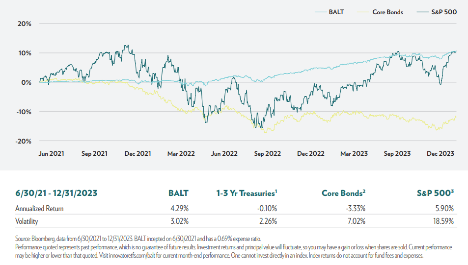
The Innovator Defined Wealth Shield ETF (BALT) seeks to track the return of the SPDR S&P 500 ETF Trust (SPY), to a cap, and provide a measure of downside protection by seeking to buffer investors against losses. The ETF targets a 20% buffer for every 3-month outcome period. The ETF can be held indefinitely, resetting at the end of each outcome period. BALT has an annual expense ratio of 0.69%.
BALT is designed to be a defensive investment that seeks to offer a built-in buffer against downside losses while providing upside return potential to a cap, over each quarterly outcome period.
What are the potential benefits of a Buffer ETF with a 3-month reset?
Potential Benefits:
• Upside exposure of U.S. equities to a cap, with a 20% buffer against losses every quarter
• Defined outcome parameters
• Hedged equity risk with a potentially more attractive upside than bonds
• Historical volatility more in line with bonds than equities, without taking on interest rate risk
• The potential for a greater level of downside protection with a 20% buffer over a shorter time period
• Potential alternative to bonds
• Rebalances quarterly and can be held indefinitely
• Tax efficient
• Liquid and transparent
• No credit risk
BALT holds a customized basket of FLEX options with the same expiration date (approximately three months), but with varying strike prices. In combination, these options give BALT a defined buffer level and upside growth potential to a cap, over its outcome period. BALT is designed to roll into a new basket of FLEX options at the end of each quarterly outcome period. BALT’s three-month buffer against losses is targeted to be 20%.
Like other Buffer ETFs, BALT does not have a maturity date. Upon the conclusion of the outcome period, BALT will roll into a new portfolio of FLEX options with the same reference asset (SPY) and term (three months), with a fresh buffer and new upside cap. BALT can therefore be held as a long-term investment.
BALT may appeal to investors who are looking for an investment with a defensive profile that is similar to that of bonds, but typically offers higher upside potential than bonds. Note, BALT does not pay income.
The funds have characteristics unlike many other traditional investment products and may not be suitable for all investors. For more information regarding whether an investment in the fund is right for you, please see “Investor Suitability” in the prospectus. The fund does not provide investment income and loss of principal is possible.
Cumulative Returns: BALT vs. Stocks and Core Bonds (6/30/2021 – 12/31/2023)
Innovator also offers a 10% Buffer ETF that resets every three months. Innovator U.S. Equity 10 Buffer ETF (ZALT) seeks to track the return of the SPDR S&P 500 ETF Trust (SPY), to a cap, and provide a measure of downside protection by seeking to buffer investors against losses. The ETF targets a 10% buffer for every 3-month outcome period. The ETF resets at the end of each outcome period and can be held indefinitely. ZALT has an annual expense ratio of 0.69%.
ZALT is essentially the equivalent of BALT, but with a 10% quarterly buffer. The reduced amount of downside protection will typically allow ZALT to have a higher quarterly upside cap.
ZALT was listed for trading on October 2, 2023. The first outcome period for a cap comparison with BALT was January 1, 2024. ZALT, which offers approximately half as much downside protection as BALT each quarter (10% vs. 20%), had an upside gross cap of 3.23% vs. 2.56% for BALT. This is approximately 26% higher over the 3-month period. On an annualized basis, assuming the cap difference stays the same throughout 2024, ZALT would offer an extra 2.68% upside return potential over a 12-month period, but again, with half the downside protection each quarter.
Both BALT and ZALT are defensive Buffer ETFs that offer the potential to outperform bonds and could serve as a bond complement in a portfolio.
Most Buffer ETFs are perpetual products that are designed to rebalance on the reset date. At the beginning of each outcome period the ETFs are set with defined parameters, a known cap level and downside buffer, typically over a one-year outcome period. At the end of each outcome period the ETF will rebalance into a new outcome period.
The rebalance is simple and consists of the ETF taking the proceeds of the expiring basket of options and reinvesting into a new set of options that will construct the new outcome parameters for the next outcome period. This is all done simultaneously and the rebalance does not typically create a taxable event.
Expiring options are replaced with new options
At the end of each outcome period (reset date), the four option contracts in the Buffer ETF wrapper expire automatically. The proceeds from the expiring options roll into a new basket of four option contracts for the next outcome period.
Most Buffer ETF issuers rebalance on the last business day of the month, at the end of the outcome period. However, FT Vest typically rebalances on the third Friday of the month, which corresponds with options expiration. On the reset date, a package of four option contracts is auctioned off to market makers. The options are packaged together and the highest bid from the market makers determines the cap level for the next outcome period. The cap level is the only variable on the reset date and it’s heavily influenced by market volatility and interest rates.
Considerations:
Index level: The new defined outcome parameters are based on the traded reference asset price level.
NAV: The NAV (net asset value) at the end of the outcome period is also the beginning NAV for the new outcome period.
Cap and Buffer: The new cap and buffer are based on the reference asset price level and the final NAV.
New Outcome Period Parameters: The new parameters take effect at the close of the last trading day of the outcome period. When the market opens on the first trading day of the new outcome period, the new parameters are already in place.
Buffer ETFs are somewhat complex, but if we peel back the ETF wrapper to look inside on the reset date, we can better understand how they work. And, by defining the role of each of the four option positions within the ETF wrapper, we can more easily understand how the downside buffer and upside cap are created (and the costs involved) at the beginning of the outcome period.
As you know, the buffer provides a protective layer designed to absorb a specific percentage of losses over a defined outcome period. Think of it as protection that shields an investor’s portfolio down to a certain level during the outcome period, which is typically 12 months. For example, the 15% buffer provided by Innovator’s U.S. Equity Power Buffer – November series (PNOV), is designed to protect an investor against the first 15% loss of the reference asset. If the buffer level is breached at the end of the outcome period, an investor would experience a loss on the position. This assumes a purchase on the reset date. Intra-outcome purchases will have different defined outcome parameters.
A Buffer ETF strategy is achieved by using four different FLEX options, which are uniquely versatile due to their customizable nature. They allow the ETF issuer to tailor protection and outcome parameters.
In the table you can see inside the ETF wrapper of PNOV after the market’s close on the reset day, October 31, 2022. These are the holdings and outcome parameters for the new outcome period, which begins on November 1.
| Date | Ticker | Transaction | Security Name | Shares | Price | Market Value | Weighting | Layer | Notes |
| 10/31/22 | PNOV | Buy call | SPY 10/31/2023 3.86 C | 8283 | 375.79 | $311,266,857.00 | 98.06% | 1 | 1:1 S&P 500 ETF Upside |
| 10/31/22 | PNOV | Sell call | SPY 10/31/2023 465.46 C | -8283 | 10.53 | ($8,721,999.00) | -2.75% | 3 | 20.5% Upside Cap |
| 10/31/22 | PNOV | Sell put | SPY 10/31/2023 328.28 P | -8283 | 14.48 | ($11,993,784.00) | -3.78% | 2 | 15% Buffer |
| 10/31/22 | PNOV | Buy put | SPY 10/31/2023 386.21 P | 8283 | 31.56 | $26,141,148.00 | 8.24% | 2 | 15% Buffer |
| 10/31/22 | Cash & Other | 1.0 | $693,079.91 | 0.22% | Cash | ||||
| Net Assets | $317,411,797.50 |
Definitions:
Ticker: Buffer ETF trading symbol
Transaction: Purchase or sale of option contracts
Security: Option contracts purchased or sold
Shares: Number of shares
Price: Cost of the security
Market Value: Dollar value of the purchase or sale of the option contract
Weighting: Percentage weighting of each security held in the ETF
Net Assets: Net dollar amount held in the ETF following the reset
Layer 1: Buy a call option to provide synthetic 1:1 exposure to the reference asset (SPY). A synthetic investment is designed to replicate the return of a selected index.
Layer 2: A) Buy a put option to provide downside protection on the reference asset. B) Sell a put option (to help fund the purchase of the protective put) with a strike price at the level where the protection will end (-15%).
Layer 3: Sell a call option (to help fund the purchase of the protective put). The premium received from the sale of this call option will determine the cap level during the outcome period. Any gain of the reference asset that surpasses the upside cap will be effectively forfeited by the investor. This is the cost of having a level of protection in place during the outcome period.
Understanding the role of each option layer:
Layer 1
On the reset date, a call option was purchased that provided synthetic 1:1 exposure to the reference asset (SPY) that PNOV is designed to track. 98.06% of the available cash in the ETF on the reset date was used to purchase this call option. It cost $311,266,857 to provide the exposure to the reference asset.
Layer 2
Layer 2 is a put spread – a purchase and a sale of a put option. Together the long and short put create the buffer, ensuring protection against initial losses. The purchase of the put provides downside protection for the approximately $311 million that was invested to track the reference asset. Note, for PNOV, the purchase of the put provided downside protection from the current price of SPY, $386.21 to $328.28, which is approximately 15% below the current price.
The cost of the protective put was $26,141,148. This dollar amount, plus the cost of the call option in Layer 1, means there is now a dollar deficit in the ETF. There’s not enough money to pay for the purchase of the options. So, the ETF must sell options (collect premiums) to offset the cost of the protective put.
The second option position in Layer 2 involves the sale of a put with a strike price at $328.28. This sale helps fund the cost of the protective put and it also determines where the downside protection will end. So, if the buffer is exhausted at the end of the outcome period, any further loss in SPY will see the Buffer ETF’s value decrease by the same percentage (1:1). The strike price is 15% below the current level of the reference asset ($386.21 – $328.28 = $57.93). 57.93/386.21 = 15%. The sale of the put option raised $11,993,784 in a premium that will be used to partially pay for the purchase of the put option.
Again, if the reference asset falls by 15%, the put spread will protect against the loss. However, because the ETF sold a put option with a strike price 15% below the current level of SPY on the reset date, it means the investor will no longer have protection if the 15% loss level is breached at the end of the outcome period (12 months later). The ETF shareholder will participate 1:1 in any loss greater than 15%. For example, if the reference asset falls 25% at the end of the outcome period, the ETF would lose 10% (before fees).
Layer 3
The third and final layer of the options strategy is a sale of a call option on the reference asset. With this sale the ETF receives the call premium and it also establishes an upside cap. The cap determines the maximum potential gain for the Buffer ETF during the outcome period.
The premium received from the sale of the call option will help fund the purchase of the protective put option in Layer 2. Again, the sale of the call option “caps” the return of the ETF during the outcome period. The call option in PNOV was sold at $465.46. This was approximately 20.5% above the price of the reference asset (SPY) on the reset date. If the reference asset gained more than 20.5% at the end of the outcome period, a PNOV shareholder would effectively forfeit the additional gains. A shareholder’s maximum gain over the outcome period is capped at 20.5% (before fees), due to the sale of the call option. The option sale was necessary to help fund the cost of the protective put in Layer 2.
How are the new options purchased and sold on the reset date?
The four option contracts from the previous 12-month outcome period expire automatically. The assets in the ETF then roll into a new basket of options containing four contracts for the next outcome period. On the reset date, a package of the four option contracts is auctioned off to market makers. The options are not bought or sold separately, rather, they are packaged together. Once the highest bid is known, the cap level is determined for the upcoming outcome period. The upside cap level is the only unknown heading into each reset date. The buffer level remains the same as all prior outcome periods and the reference asset is the same too, but the level of the upside cap will change. The cap level is typically influenced by both interest rates and volatility in the options market.
Note: A discerning reader may have noticed in the table of PNOV on its reset date, the premiums received from the sales of the put and call options did not fully cover the cost of the protective put. The protective put cost $26,141,148.00, but the sale of the put and call options only raised $20,715,783 ($8,721,999.00 + $11,993,784.00). So, there is a deficit of $5,425,365. How is there enough cash in the ETF to pay for the total cost of the protective put? Well, the purchase of the call option in Layer 1 was done at a “discounted” price that was basically ex-dividend on the reference asset (SPY). Buffer ETFs don’t pay dividends, so the call buyer effectively gets a discounted price on the options by the dollar amount of the dividends that will be paid during the outcome period. The annual dividend yield on SPY was approximately 1.7% on the reset date, which adds up to a little over $5 million, effectively covering the deficit in the ETF.
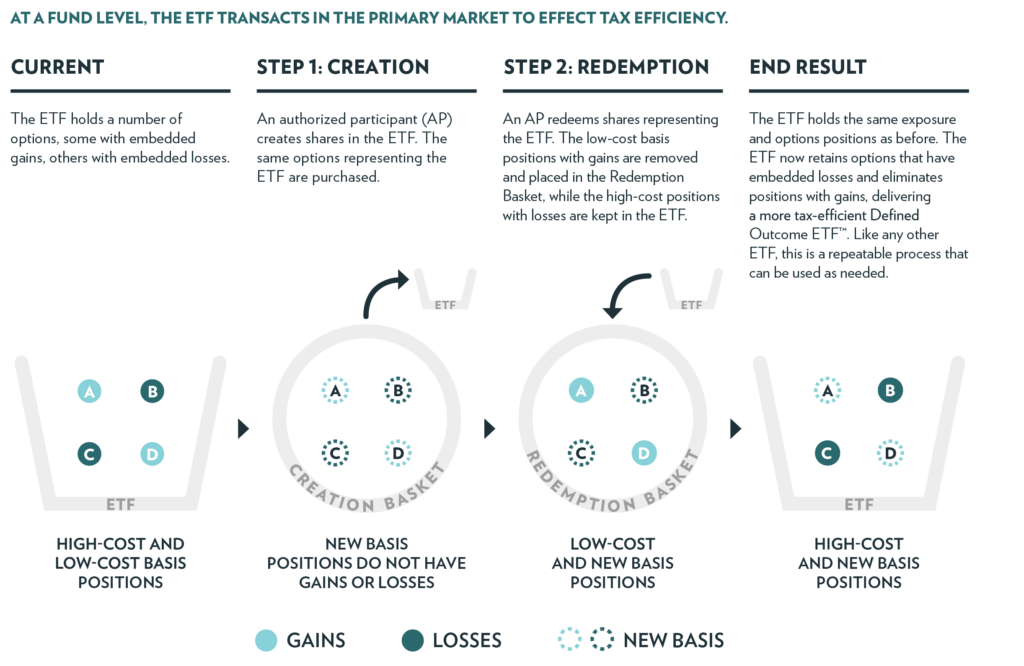
The same benefits of the ETF creation/redemption process that make stock and bond ETFs more tax efficient can also be utilized with Buffer ETFs. Through the creation/redemption process, the ability to redeem gains and keep losses in the portfolio should allow Buffer ETFs to be as tax efficient as traditional ETFs.
• Tax deferral until sold
• No anticipated capital gains distributions to shareholders
• Potential alternative to structured notes or annuities
The creation/redemption process that allows for tax efficiency with Buffer ETFs can be visualized below:
An important white paper from Dr. Joanne M. Hill was recently published in the Journal of Beta Investment Strategies (Winter 2023). Her findings, in the study titled Evaluating Target Performance for Downside Buffer ETFs, show how successful the primary issuers of Buffer ETFs have been at hitting their published return targets during the outcome periods.
In the study, Dr. Hill assessed how Buffer ETFs have delivered on their goal of achieving their target returns for various outcome periods. Dr. Hill analyzed the tracking experience of the ETFs compared to the returns of the reference asset, net of management fees. The study provides insight into how well Buffer ETFs have accomplished the investment objectives that were disclosed at the start of each outcome period, in terms of the downside buffer and upside cap.
Key Findings:
• By evaluating a large sample of Buffer ETFs over a range of equity market conditions, the study shows that Buffer ETF managers have broadly delivered on their promise to provide a targeted return over a defined outcome period.
• The return range relative to the benchmark has been consistent over the past several years, and has averaged close to 0%, with a standard deviation of less than 0.20%.
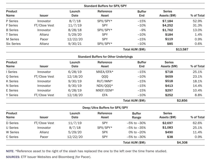
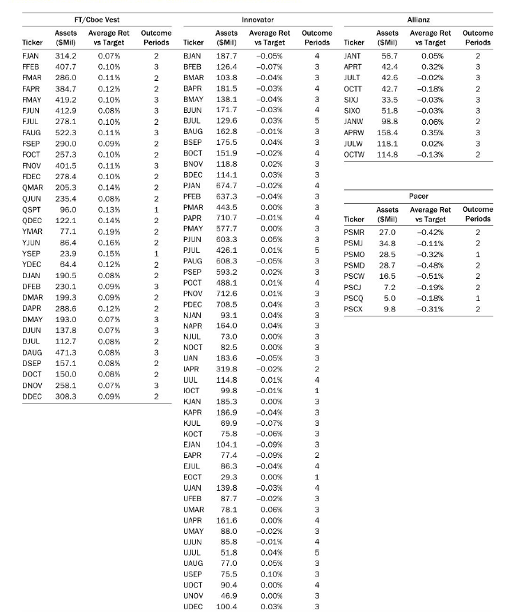
To have a broad sample of outcome periods, the study shows data only from Buffer ETF issuers with at least six reset periods. This restricted the sample to four issuers: Innovator, FT Cboe Vest, Allianz, and Pacer. The sample of 102 ETFs is listed at the end of this section and encompasses almost $21 billion in assets, or approximately 80% of the total Buffer ETF assets. The table shows the full set of Buffer ETF series studied, along with their issuers, assets as of June 30, 2023, and launch dates.
Series of Standard and Deep Buffer ETF Series – Assets, Issuer and Launch Date
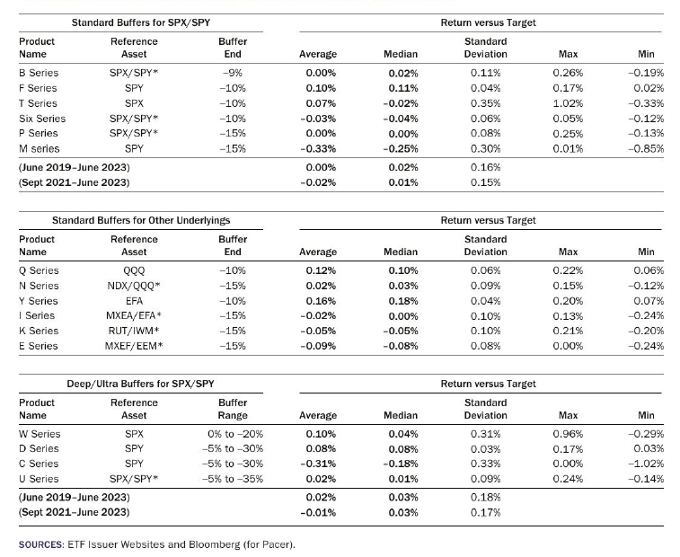
The table shows a summary of the Tracking Metrics for various Buffer ETF series. The difference between the Buffer ETF return and the target return for each series is averaged across the different reset periods. The standard deviation is also shown to help assess the variability of tracking errors. The Buffer ETFs with SPY as the reference asset showed the overall average tracking difference was close to zero (slightly positive), and the standard deviation across all series was under 0.20%, showing relatively tight tracking versus the targets.
Tracking Metrics for Standard and Deep Buffer ETF Series (as of June 30, 2023)
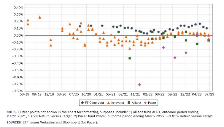
The chart shows consistency of tracking by examining a scatter plot of results over time. Investors can assess the range and consistency of ETF returns across all series. “The scatter plot shows the variations in benchmark tracking have been relatively consistent over time since 2021 for Innovator and FT Cboe Vest, with most tracking within 0.20% of the benchmark. Allianz and Pacer’s Buffer ETF returns versus the Target Performance Benchmark have been more variable but have narrowed over time.”
Return-Target: Buffer ETF Series with SPX/SPY Underliers (June 2019 to June 2023)
Summary: Dr. Hill’s study assessed how well Buffer ETFs have performed relative to their target returns that were disclosed to investors at the start of each outcome period. For a large sample of Buffer ETFs with reference assets of SPY, QQQ, IWM, EFA, and EEM from four different issuers, the analysis showed that the return tracking range has been very consistent over time. Overall, the results show that investors should have a high degree of confidence that Buffer ETFs will deliver the expected outcomes during a wide range of market conditions.
Tracking by Buffer ETF Ticker Across Various Outcome Periods since Launch
What are Buffer ETFs?
Buffer ETFs are revolutionary products that provide a range of potential outcomes to investors before they invest. These differ from undefined ETFs by setting parameters to the upside and downside. The ETFs offer exposure to the price return of a reference asset (either a broad market ETF or index) to a cap, typically over a three-month, six-month, or one-year outcome period, at which point each ETF will reset. Historically, these types of defined outcome strategies have only been available through structured notes and certain insurance products.
How do Buffer ETFs work?
Each Buffer ETF holds a customized basket of FLEX options with varying strike prices (the price at which the option purchaser may buy or sell the security at the expiration date) and the same expiration of typically one year. This gives each ETF a defined buffer level and upside growth potential (to a cap), over an outcome period. Each ETF intends to roll options components on the reset date, which is typically on the last business day of the month associated with each ETF. Note, FT Vest rolls options on the third Friday of the month, which corresponds with options expiration.
How are Buffer ETFs created?
Buffer ETFs are typically created with FLEX options. FLEX options offer customized terms of an option, including strike prices, underlying reference assets and expiration dates. They also trade on an exchange, listed on the Chicago Board Options Exchange, and are backed by the Options Clearing Corporation (OCC).
The OCC is guarantor and central counterparty with respect to options. As a result, the ability of a Buffer ETF to meet its objective depends on the OCC being able to meet its obligations.
Designated as a Systemically Important Financial Market Utility (SIFMU), the OCC has heightened risk management and liquidity standards, significantly reducing counterparty risk. Buffer ETFs are not backed by the credit of an issuing institution and therefore are not subject to credit risk.
What are the benefits of the ETF wrapper?
Intraday liquidity, pricing transparency, and tax efficiency are just a few of the benefits derived from the ETF structure.
What are the expense ratios?
Most Buffer ETFs have annual expense ratios of approximately 0.80%. However, there are some Buffer ETF offerings with annual expense ratios of 0.50%. See the section titled Buffer ETF Offerings for more information.
What if I buy shares of a Buffer ETF after the reset date?
Investors purchasing shares of a Buffer ETF after its reset date may receive a different payoff profile than those who purchased the ETF on the reset date. However, investors purchasing shares after the first day will still be able to know their potential outcomes, no matter when they invest during the one-year period, based on the current ETF price and the length of time remaining before expiration. Visit the issuing company’s website to see the potential outcome parameters before investing.
If I buy shares of a Buffer ETF at its initial price on the first day of trading, at the end of the outcome period, can I expect to participate in the upside of the reference asset to a cap, with a downside buffer level, before fees and expenses?
Yes. These ETFs are designed to provide point-to-point exposure to the price return of the reference asset. They are not expected to move precisely in line with each respective reference asset during the outcome period (due to the optionality of the underlying portfolio). It is also important to note that there is no assurance that Buffer ETFs will meet their investment objectives.
Does a Buffer ETF mature?
No. Upon the conclusion of the outcome period, the ETF will automatically reset into a new portfolio with the same exposure, buffer level, and term, and a new upside cap will be determined.
Does any entity guarantee I will not lose my investment?
No. Unlike certain insurance products and structured products, ETFs are not backed by the faith and credit of an issuing institution like an insurance company or a bank. This also means that Buffer ETFs are not exposed to credit risk. The options held by the ETFs are guaranteed for settlement by the Options Clearing Corporation (OCC). In the unlikely event the OCC becomes insolvent or is otherwise unable to meet its settlement obligations, the ETFs could suffer significant losses. However, regulators have heightened their oversight of the OCC due to its designation as a Systemically Important Financial Market Utility (SIFMU).
Are there any comparable products that exist in the market?
Buffer ETFs are designed to offer investors more efficient, cost-effective, and more accessible alternatives to structured notes and certain insurance products. While those products can play an important role in certain investors’ portfolios, characteristics like high fees, illiquidity, lack of transparency, and counterparty risk have set the stage for an alternative, such as Buffer ETFs. Many of the benefits of defined outcome products can be harnessed efficiently and cost-effectively in an ETF wrapper.
Buffer ETFs appeal to what type of investor?
The ability to know potential outcome parameters before investing has countless applications. Buffer ETFs appeal to a variety of investors seeking stock market growth, to a cap, with a downside buffer. These may include conservative or moderate-risk investors, pre-retirees, and retirees.
Can an investor buy and hold a Buffer ETF, or do they need to repurchase the ETF each year?
Buffer ETFs automatically reset at the conclusion of their respective outcome periods and may be held indefinitely. At the end of an outcome period, each ETF will roll into a new set of options contracts with the same exposure, buffer level, and term length, and a new upside cap will be determined.
Are Buffer ETFs a good fit for my portfolio?
Buffer ETFs can be used as a complement or replacement for both equity and fixed income allocations in existing portfolios. The liquidity, transparency, and tax efficiency now afforded to structured outcomes, make Buffer ETFs an attractive addition to a portfolio.
Are there benefits to Buffer ETFs over structured products and indexed annuities?
Buffer ETFs attempt to solve several issues often associated with structured products that seek to provide investors with known return profiles: liquidity risk and counterparty credit risk. Buffer ETFs are fully transparent and more flexible than the typical structured products you might find in the marketplace.
When can I trade?
Buffer ETFs invest and capture market exposure in the deepest, most liquid markets in the world. Buffer ETFs allow investors to trade in large sizes at competitive prices. It is critical to remember that liquidity of an ETF is driven by the underlying exposure held by the ETF, not the ETF itself.
Investors can buy and sell Buffer ETFs just like any other ETF. These ETFs are actively traded during market hours. Furthermore, unlike traditional structured products, investors can buy and sell at any point during an outcome period. Investors can also remain confident that their execution will be consistent due to the deep liquidity profile underlying the Buffer ETFs. The tradability of Buffer ETFs is yet another benefit of the ETF structure, and it allows investors to transact with ease.
If an investor decides to transact intra-outcome period, the potential outcome parameters can be viewed on the issuer’s website.
When should I trade?
While investors may initiate a position at any point during an outcome period, activity tends to be highest around the reset date for Buffer ETFs. Why is this the case? Investors who purchase and hold these ETFs from the start to the end of an outcome period will receive the stated cap and buffer levels. Investors who purchase after the first day of an outcome period will also experience a defined outcome, but with different cap and buffer levels. For investors seeking the stated cap and buffer, it’s recommended they initiate a position in the final hours of trading on the reset date (the day before the new outcome period begins).
What if I see low volume on a Buffer ETF prior to entering an order?
Low volume should be of no concern. An ETF’s liquidity is derived from the liquidity of its underlying components. Buffer ETFs track the largest and most well-known underlying indices, so there is considerable liquidity underlying each of the ETFs. If desired, an investor can always enter a limit order for a purchase or sale.
Is there a minimum or maximum order size?
No.
Buffer ETF Definitions:
Reference asset exposure: the reference asset the ETFs are providing structured exposures to.
Upside Cap: the maximum potential return, before fees and expenses, if held to the end of the current outcome period. The ETF does not participate in growth beyond the cap.
Buffer: the amount of downside protection, before fees and expenses, the fund seeks to provide, over the full outcome period.
Outcome Period: the intended length of time over which the defined outcomes are sought. The remaining terms are applicable to those considering an investment in an ETF during the outcome period.
Remaining Upside Cap: the current maximum return available at the ETF’s current price, before fees and expenses, if held to the end of the outcome period. Remaining upside cap is a function of the ETF’s return, not the return of the index.
Remaining Downside Buffer: the current amount of downside buffer remaining at the ETF’s current price, before fees and expenses, if held to the end of the outcome period.
Downside Before Buffer: the amount of ETF loss incurred before the buffer begins. This is applicable to investors considering a purchase or sale during the outcome period.
Remaining Outcome Period: the number of days remaining until the last day of the outcome period.
Fees and Expenses: the ETF’s management fees, any shareholder transaction fees and any extraordinary expenses.
Option Definitions:
Call Option: a call option gives the buyer the right to buy an asset at a specified price.
Put Option: a put option gives the buyer a right to sell an asset at a specified price.
Strike Price: the agreed-upon price at which an underlying asset can be bought or sold.
At-the-Money: an option is at-the-money if the strike price and price of the underlying asset are equal.
In-the-Money: an option that possesses intrinsic value. An option that’s in-the-money is an option that presents a profit opportunity due to the relationship between the strike price and the prevailing market price of the underlying asset.
In-the-Money Call Option: the option holder can buy the security below its current market price.
In-the-Money Put Option: the option holder can sell the security above its current market price.
Out-of-the-Money: a call option is out-of-the-money if the underlying price is trading below the strike price of the call. A put option is out-of-the-money if the underlying price is above the put’s strike price.